Spaces:
Sleeping
Sleeping
| #!/usr/bin/env python | |
| # coding: utf-8 | |
| # # Data integration and batch correction | |
| # | |
| # An important task of single-cell analysis is the integration of several samples, which we can perform with omicverse. | |
| # | |
| # Here we demonstrate how to merge data using omicverse and perform a corrective analysis for batch effects. We provide a total of 4 methods for batch effect correction in omicverse, including harmony, scanorama and combat which do not require GPU, and SIMBA which requires GPU. if available, we recommend using GPU-based scVI and scANVI to get the best batch effect correction results. | |
| # | |
| # | |
| # In[1]: | |
| import omicverse as ov | |
| #print(f"omicverse version: {ov.__version__}") | |
| import scanpy as sc | |
| #print(f"scanpy version: {sc.__version__}") | |
| ov.utils.ov_plot_set() | |
| # ## Data integration | |
| # | |
| # First, we need to concat the data of scRNA-seq from different batch. We can use `sc.concat` to perform it。 | |
| # | |
| # The dataset we will use to demonstrate data integration contains several samples of bone marrow mononuclear cells. These samples were originally created for the Open Problems in Single-Cell Analysis NeurIPS Competition 2021. | |
| # | |
| # We selected sample of `s1d3`, `s2d1` and `s3d7` to perform integrate. The individual data can be downloaded from figshare. | |
| # | |
| # - s1d3: | |
| # - s2d1: | |
| # - s3d7: | |
| # In[2]: | |
| adata1=ov.read('neurips2021_s1d3.h5ad') | |
| adata1.obs['batch']='s1d3' | |
| adata2=ov.read('neurips2021_s2d1.h5ad') | |
| adata2.obs['batch']='s2d1' | |
| adata3=ov.read('neurips2021_s3d7.h5ad') | |
| adata3.obs['batch']='s3d7' | |
| # In[3]: | |
| adata=sc.concat([adata1,adata2,adata3],merge='same') | |
| adata | |
| # We can see that there are now three elements in the batch | |
| # In[4]: | |
| adata.obs['batch'].unique() | |
| # In[7]: | |
| import numpy as np | |
| adata.X=adata.X.astype(np.int64) | |
| # ## Data preprocess and Batch visualize | |
| # | |
| # We first performed quality control of the data and normalisation with screening for highly variable genes. Then visualise potential batch effects in the data. | |
| # | |
| # Here, we can set `batch_key=batch` to correct the doublet detectation and Highly variable genes identifcation. | |
| # In[8]: | |
| adata=ov.pp.qc(adata, | |
| tresh={'mito_perc': 0.2, 'nUMIs': 500, 'detected_genes': 250}, | |
| batch_key='batch') | |
| adata | |
| # We can store the raw counts if we need the raw counts after filtered the HVGs. | |
| # In[10]: | |
| adata=ov.pp.preprocess(adata,mode='shiftlog|pearson', | |
| n_HVGs=3000,batch_key=None) | |
| adata | |
| # In[11]: | |
| adata.raw = adata | |
| adata = adata[:, adata.var.highly_variable_features] | |
| adata | |
| # We can save the pre-processed data. | |
| # In[12]: | |
| adata.write_h5ad('neurips2021_batch_normlog.h5ad',compression='gzip') | |
| # Similarly, we calculated PCA for HVGs and visualised potential batch effects in the data using pymde. pymde is GPU-accelerated UMAP. | |
| # In[13]: | |
| ov.pp.scale(adata) | |
| ov.pp.pca(adata,layer='scaled',n_pcs=50,mask_var='highly_variable_features') | |
| adata.obsm["X_mde_pca"] = ov.utils.mde(adata.obsm["scaled|original|X_pca"]) | |
| # There is a very clear batch effect in the data | |
| # In[14]: | |
| ov.utils.embedding(adata, | |
| basis='X_mde_pca',frameon='small', | |
| color=['batch','cell_type'],show=False) | |
| # ## Harmony | |
| # | |
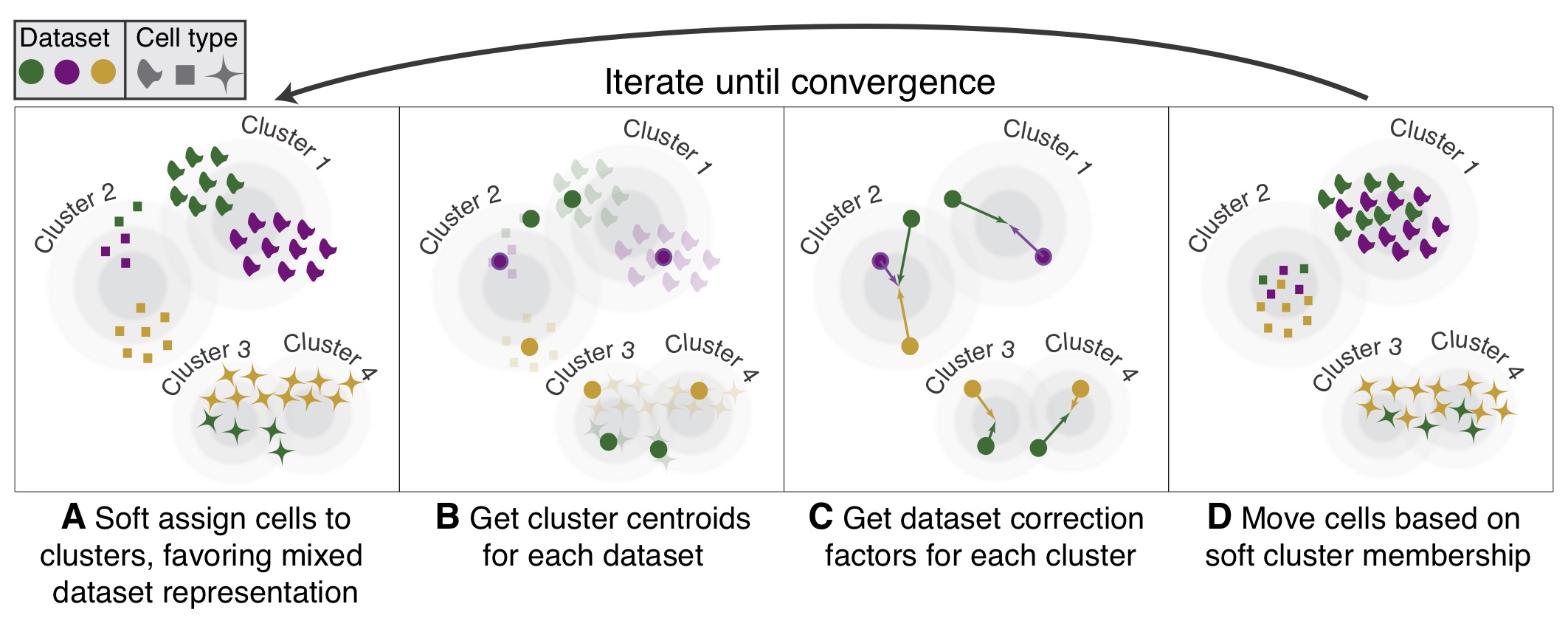
| # Harmony is an algorithm for performing integration of single cell genomics datasets. Please check out manuscript on [Nature Methods](https://www.nature.com/articles/s41592-019-0619-0). | |
| # | |
| #  | |
| # The function `ov.single.batch_correction` can be set in three methods: `harmony`,`combat` and `scanorama` | |
| # In[40]: | |
| adata_harmony=ov.single.batch_correction(adata,batch_key='batch', | |
| methods='harmony',n_pcs=50) | |
| adata | |
| # In[41]: | |
| adata.obsm["X_mde_harmony"] = ov.utils.mde(adata.obsm["X_harmony"]) | |
| # In[42]: | |
| ov.utils.embedding(adata, | |
| basis='X_mde_harmony',frameon='small', | |
| color=['batch','cell_type'],show=False) | |
| # ## Combat | |
| # | |
| # combat is a batch effect correction method that is very widely used in bulk RNA-seq, and it works just as well on single-cell sequencing data. | |
| # | |
| # | |
| # In[43]: | |
| adata_combat=ov.single.batch_correction(adata,batch_key='batch', | |
| methods='combat',n_pcs=50) | |
| adata | |
| # In[44]: | |
| adata.obsm["X_mde_combat"] = ov.utils.mde(adata.obsm["X_combat"]) | |
| # In[45]: | |
| ov.utils.embedding(adata, | |
| basis='X_mde_combat',frameon='small', | |
| color=['batch','cell_type'],show=False) | |
| # ## scanorama | |
| # | |
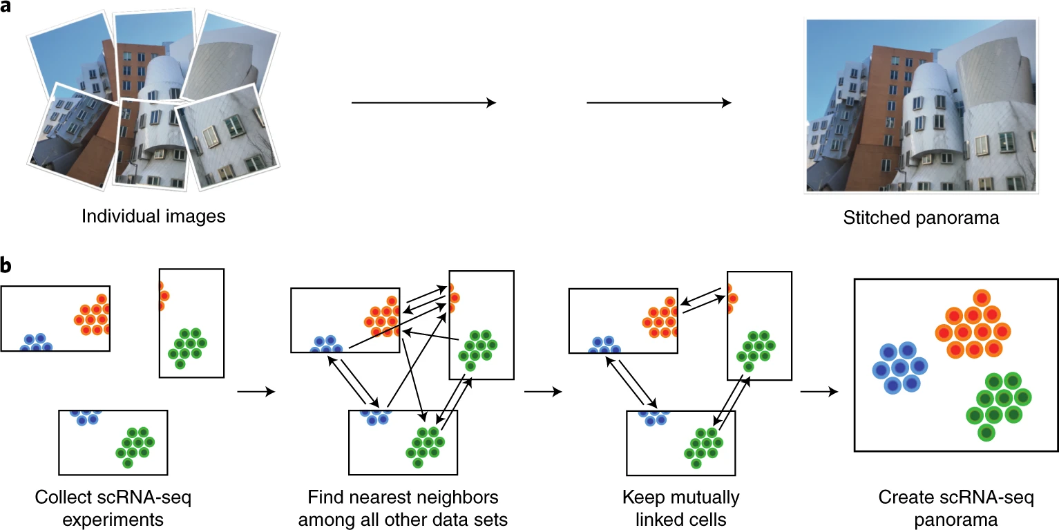
| # Integration of single-cell RNA sequencing (scRNA-seq) data from multiple experiments, laboratories and technologies can uncover biological insights, but current methods for scRNA-seq data integration are limited by a requirement for datasets to derive from functionally similar cells. We present Scanorama, an algorithm that identifies and merges the shared cell types among all pairs of datasets and accurately integrates heterogeneous collections of scRNA-seq data. | |
| # | |
| #  | |
| # In[46]: | |
| adata_scanorama=ov.single.batch_correction(adata,batch_key='batch', | |
| methods='scanorama',n_pcs=50) | |
| adata | |
| # In[47]: | |
| adata.obsm["X_mde_scanorama"] = ov.utils.mde(adata.obsm["X_scanorama"]) | |
| # In[48]: | |
| ov.utils.embedding(adata, | |
| basis='X_mde_scanorama',frameon='small', | |
| color=['batch','cell_type'],show=False) | |
| # ## scVI | |
| # | |
| # An important task of single-cell analysis is the integration of several samples, which we can perform with scVI. For integration, scVI treats the data as unlabelled. When our dataset is fully labelled (perhaps in independent studies, or independent analysis pipelines), we can obtain an integration that better preserves biology using scANVI, which incorporates cell type annotation information. Here we demonstrate this functionality with an integrated analysis of cells from the lung atlas integration task from the scIB manuscript. The same pipeline would generally be used to analyze any collection of scRNA-seq datasets. | |
| # In[3]: | |
| adata_scvi=ov.single.batch_correction(adata,batch_key='batch', | |
| methods='scVI',n_layers=2, n_latent=30, gene_likelihood="nb") | |
| adata | |
| # In[4]: | |
| adata.obsm["X_mde_scVI"] = ov.utils.mde(adata.obsm["X_scVI"]) | |
| # In[5]: | |
| ov.utils.embedding(adata, | |
| basis='X_mde_scVI',frameon='small', | |
| color=['batch','cell_type'],show=False) | |
| # ## MIRA+CODAL | |
| # | |
| # Topic modeling of batched single-cell data is challenging because these models cannot typically distinguish between biological and technical effects of the assay. CODAL (COvariate Disentangling Augmented Loss) uses a novel mutual information regularization technique to explicitly disentangle these two sources of variation. | |
| # In[15]: | |
| LDA_obj=ov.utils.LDA_topic(adata,feature_type='expression', | |
| highly_variable_key='highly_variable_features', | |
| layers='counts',batch_key='batch',learning_rate=1e-3) | |
| # In[16]: | |
| LDA_obj.plot_topic_contributions(6) | |
| # In[17]: | |
| LDA_obj.predicted(15) | |
| # In[37]: | |
| adata.obsm["X_mde_mira_topic"] = ov.utils.mde(adata.obsm["X_topic_compositions"]) | |
| adata.obsm["X_mde_mira_feature"] = ov.utils.mde(adata.obsm["X_umap_features"]) | |
| # In[38]: | |
| ov.utils.embedding(adata, | |
| basis='X_mde_mira_topic',frameon='small', | |
| color=['batch','cell_type'],show=False) | |
| # In[39]: | |
| ov.utils.embedding(adata, | |
| basis='X_mde_mira_feature',frameon='small', | |
| color=['batch','cell_type'],show=False) | |
| # ## Benchmarking test | |
| # | |
| # The methods demonstrated here are selected based on results from benchmarking experiments including the single-cell integration benchmarking project [Luecken et al., 2021]. This project also produced a software package called [scib](https://www.github.com/theislab/scib) that can be used to run a range of integration methods as well as the metrics that were used for evaluation. In this section, we show how to use this package to evaluate the quality of an integration. | |
| # In[6]: | |
| adata.write_h5ad('neurips2021_batch_all.h5ad',compression='gzip') | |
| # In[2]: | |
| adata=sc.read('neurips2021_batch_all.h5ad') | |
| # In[7]: | |
| adata.obsm['X_pca']=adata.obsm['scaled|original|X_pca'].copy() | |
| adata.obsm['X_mira_topic']=adata.obsm['X_topic_compositions'].copy() | |
| adata.obsm['X_mira_feature']=adata.obsm['X_umap_features'].copy() | |
| # In[ ]: | |
| from scib_metrics.benchmark import Benchmarker | |
| bm = Benchmarker( | |
| adata, | |
| batch_key="batch", | |
| label_key="cell_type", | |
| embedding_obsm_keys=["X_pca", "X_combat", "X_harmony", | |
| 'X_scanorama','X_mira_topic','X_mira_feature','X_scVI'], | |
| n_jobs=8, | |
| ) | |
| bm.benchmark() | |
| # In[9]: | |
| bm.plot_results_table(min_max_scale=False) | |
| # We can find that harmony removes the batch effect the best of the three methods that do not use the GPU, scVI is method to remove batch effect using GPU. | |